Statistical Testing
University of Toronto
August 9, 2023
Scientific method
An empirical and iterative process for developing shared knowledge.
- Define a question
- Research what’s known
- Form a hypothesis
- Perform an experiment
- Analyze the data
- Interpret and discuss
Example

Background
- The idea that the mean body temperature of a healthy adult human is \(37^oC\) (or, equivalently, \(98.6^oF\)) traces back to a book published in 1868 by the German physician Carl Reinhold August Wunderlich. This book reported on his analysis of over one million temperature readings from 24,000 patients.
- Modern studies have reported lower mean body temperatures. One such study is Mackowiak et al. (1992) which took measurements of 148 healthy adults (122 males and 26 females). They found an average mean body temperature of \(36.8^oC\).
- The above headline is from a new article about a research paper by Protsiv et al. (2020) which showed an estimated decrease in body temperature of \(0.03^oC\) per birth decade (controlling for age, body weight, height, and time of day), based on data from 3 different large studies.
- The data from Mackowiak et al. (1992) was not made available, but in Shoemaker (1996), they replicated and published data that had similar statistical properties, derived from the histogram that Mackowiak et al. (1992) reported.
Data
We will use Shoemaker’s data of 130 simulated body temperature readings for 65 hypothetical males and 65 hypothetical females.
  temp sex heartrate
1 96.3   1        70
2 96.7   1        71
3 96.9   1        74
4 97.0   1        80
5 97.1   1        73
Variables
temp: temperature in degrees Fahrenheitsex: 1 = male, 2 = femaleheartrate: heart rate in beats per minute
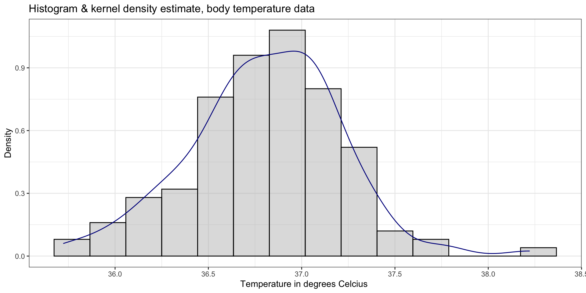
EDA

Analysis: Confidence Interval
Find a \(95\%\) confidence interval for the mean body temperature.
- Does the distribution of body temperatures look normal?
- If body temperatures \(\sim N(\mu, \sigma^2)\), do we know \(\sigma\)?
- How big is the sample size?
Recall: The studentized mean for a random distribution
\[ \frac{\bar{X}_n-\mu}{S_n/\sqrt{n}} \sim t_{n-1} \]
Formula
\[ \Pr\left( -t_{n-1,\;\alpha/2} \leq\frac{\bar{X}_n-\mu}{S_n/\sqrt{n}} \leq t_{n-1,\;\alpha/2}\right) = 1-\alpha \]
Quick exercise: Fill in the intermediate steps.
which gives this formula for a confidence interval \[ \left(\bar{x}_n - t_{n-1,\;\alpha/2} \frac{s_n}{\sqrt{n}} ,\; \bar{x}_n + t_{n-1,\;\alpha/2} \frac{s_n}{\sqrt{n}}\right) \]
Compute
 lower  upper
36.734 36.876
Does the data indicate that mean body temperature is not \(37^{\circ} C\)?
p-values
A popular type of summary statistic used when addressing hypothesis-based research questions is called a p-value.
If the parameter is what we claim, does it seem possible that we got the data that we did?
Idea
- Say we’re interested in a parameter \(\theta\) of the distribution of \(X_i\)’s.
- We think the parameter might have a particular value, call it \(\theta_0\).
- Does the data support this hypothesis?
Example: Body temperatures
- Parameter of interest: \(\mu\)
- Claim that \(\mu = \mu_0\) where \(\mu_0 = 37^{\circ} C\)
Terminology
- null hypothesis: \(H_0:\theta=\theta_0\)
- alternative hypothesis: \(H_a : \theta \neq \theta_0\)
- test statistic, \(T(X)\), is a function of the random sample and depends on \(\theta_0\)
Example: Body temperatures
- \(H_0 : \mu=37\)
- \(H_a : \mu\neq37\)
- For a t-test: \(T(X)=\frac{\bar{X}_n-\mu_0}{S_n/\sqrt{n}}\)
Definition
Assuming that \(\theta_0\) is the true value of \(\theta\), the p-value is the probability of observing the test statistic or something more extreme.
We will define a p-value as \[ p_o={\Pr}_{\theta_0}\left(\left|T(X) \right| \geq \left| t_{obs}\right| \right) \] where \(t_{obs}=T(x)\)
Example: Body temperatures
If the claim is true, then the test stat is an observation from a t-distribution with \(n-1\) degrees of freedom. What is the probability of getting the observed test statistic, or a value that is more extreme?
Interpretation
- A large p-value means the data are consistent with the claim in the null hypothesis.
- A small p-value means the data are inconsistent with the claim in the null hypothesis.
Example: Body temperatures
- \(1.21\times 10^{-7}\) is a very small p-value.
- We have strong evidence that the mean of the distribution that generated the body temperature data is not \(37^{\circ}C\)
Statistical hypothetsis testing
What are p-values?
The p-value is the probability of obtaining a result from data that is equal to or more extreme than what was actually observed, when calculated assuming the null hypothesis is true.
- The p-value is calculated from the data. So it’s another statistic.
- Since the p-value value varies with the data, if we think of it in terms of the underlying random sample, we can talk about its distribution. So what is its probability distribution if the parameter is, indeed, what we claim?
Terminology
When we want to make {yes, no} decisions about whether the data supports a certain true value of the parameter, we call the process a statistical hypothesis test.
Very often, p-values are used in statistical hypothesis testing.
Suppose \(X_1, ..., X_n\overset{iid}{\sim} F_\theta\). We want to assess the support for the claim that \(\theta = \theta_0\).
- If we want to check a p-value against a threshold of \(\alpha\in (0,1)\), then we say we are testing the hypothesis that \(\theta = \theta_0\) at significance level \(\alpha\).
- If \(p_o<\alpha\), we “reject” the hypothesis at the \(\alpha\) level.
- Otherwise, we say that the observed data does not provide sufficient evidence to reject the hypothesis at the \(\alpha\) level.
Limitations
A small p-value can occur because
- \(\theta \neq \theta_0\)
- \(\theta = \theta_0\) but we have some very unusual data
- at least one of the assumptions of the statistical test used was violated
- A small p-value does not indicate an important departure from the null hypothesis. You may hear people say that “statistical significance does not imply practical importance”.
- A very small p-value may still indicate more support for the null than for the alternative hypothesis.
- A p-value only gives evidence against the null hypothesis. It does not give an indication of which element of the alternative might be best supported by the data.
- Beware of “bright-line” thinking.
- Use caution when imposing binary thinking on a continuous world.
- For good science, p-values should be used in conjunction with other tools and with consideration for the context.
Test statistics
If we assume the distribution of the data is Normal, then we know that these test statistics have the following distributions:
\[ \frac{\bar{X}_n-\mu}{\sigma/\sqrt{n}}\sim \text{N}\left( 0,1 \right) \quad\text{if }\sigma\text{ is known} \]
\[ \frac{\bar{X}_n-\mu}{S_n/\sqrt{n}}\sim t_{n-1} \quad\text{if }\sigma\text{ is unknown} \]
\[ \frac{\bar{X}_n-\mu}{S_n/\sqrt{n}} \;\dot{\sim} \;\text{N}\left( 0,1 \right) \quad \text{for large }n \]
Interpretation
Rough guidelines for strength of evidence:
- If \(p_0 > 0.10\) ⇒ we have no evidence against \(H_0\)
- If \(0.05 < p_0 < 0.10\) ⇒ we have weak evidence against \(H_0\)
- If \(0.01 < p_0 < 0.05\) ⇒ we have moderate evidence against \(H_0\)
- If \(0.001 < p_0 < 0.01\) ⇒ we have strong evidence against \(H_0\)
- If \(p_0 < 0.001\) ⇒ we have very strong evidence against \(H_0\)
Example
Advertisements for a particular chocolate bar claims that they have 5 peanuts in every bar. You eat one of their chocolate bars and only find 2 peanuts. So you buy 49 more chocolates bars. You find average number of peanuts per bar is 4.37 and the standard deviation is 1.28. Does the data support the claim in the ad?
Goodness of Fit
To describe how well a model fits a set of observations, we use goodness of fit tests.
Suppose we have data \(x=(x_1,...,x_n)\), which are realizations of a sample \(X=(X_1,...,X_n)\). We are interested in the claim that \(\theta=\theta_0\) where \(\theta\) is a parameter of the probability distribution of \(X_i\).
Say we have found the maximum likelihood estimate of \(\theta\), and denote it as \(\widehat{\theta}_{MLE}\).
Likelihood ratio
The likelihood ratio is defined as
\[ \Lambda(\theta_0)=\frac{L\left( \theta_0|X\right)}{L\left( \widehat{\theta}_{MLE}|X\right)} \]
\[ \; \]
Notice that \(0 \leq \Lambda(\theta_0)\leq1\)
Likelihood ratio statistic
If we assume that the MLE satisfies \(\left. \frac{\partial\ell}{\partial\theta}\right|_{\theta=\widehat{\theta}_{MLE}} = 0\), it can be shown that the sampling distribution of the MLE is asymptotically normal. It can be shown that for large \(n\),
\[ -2\log \Lambda(\theta_0) \sim \chi_1^2 \]
We say that the likelihood ratio statistic has a chi-squared distribution with one degree of freedom. The p-value for the likelihood ratio statistic is computed as
\[ p_0=\Pr\left( \chi_1^2 > -2\log \Lambda(\theta_0) \right) \]
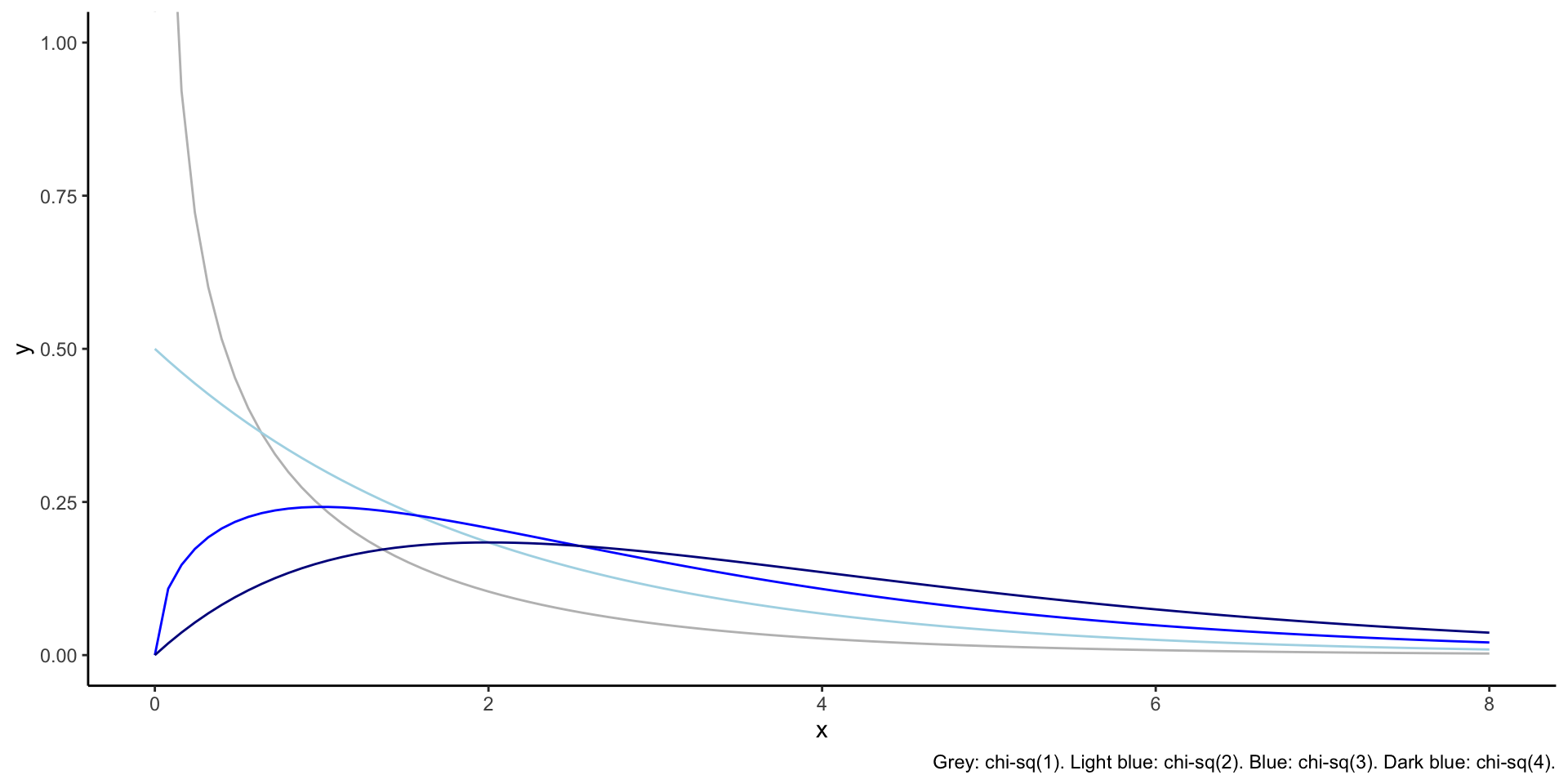
Chi-squared distribution
- One parameter, \(k\), called the degrees of freedom
- The sum of the square of \(k\) independent standard normal random variables has a \(\chi_k^2\)distribution
- For \(k=1\), support is \(x\in(0,\infty)\). For \(k>1\), support is \(x\in[0,\infty)\).
- It is right-skewed. The amount of skew decreases with k.
- It is a special case of the Gamma distribution. \[ X\sim\chi_k^2 \iff X\sim\Gamma\left(\alpha=\frac{k}{2},\beta=2\right) \]
Plots

Example
Suppose we flip a coin 50 times and get 20 heads. Is this evidence that the coin is unfair?
n <- 50
xsum <- 20

# Claim:
p0 <- 0.5

# Estimate:
p_mle <- xsum / n

# Define the log likelihood function
likelihoodfcn <- function(p){
  p^(xsum) * (1-p)^(n-xsum)
}

# Compute the likelihood ratio
LR <- likelihoodfcn(p0) / likelihoodfcn(p_mle)

# Do a likelihood ratio test to check if the data supports the claim
lr <- -2*log(LR)
1 - pchisq(lr, df = 1)
[1] 0.1559Degrees of freedom
If \(\theta \in \mathbb{R}^d\) for \(d>1\) and \(\theta = \theta_0\), then for large \(n\),
\[ -2\log \Lambda(\theta_0) \sim \chi_{d-1}^2 \]
Example: The supplemental text shows how to test a claim that digits in a dataset have been generated uniformly.
The degrees of freedom in the chi-squared distribution depend on the difference between in the degrees of freedom in the MLE and in the degrees of freedom in the hypothesis.