The Bootstrap

Sonia Markes

University of Toronto

July 26, 2023

Motivation

Sampling distributions

Recall: The Central Limit Theorem states that the sampling distribution of the sample mean is approximately normal for large \(n\). That is,

\[ \bar{X}_n \overset{D}{\longrightarrow}Y \;\; \text{where} \;\; Y\sim \text{N}\left( \mu,\frac{\sigma^2}{n} \right) \]

If \(\widehat\mu = \bar{X}_n\) where \(\mu= \mathbb{E}[X_i]\) and \(\sigma^2=Var(X_i)\), then the sampling distribution of is given by the CLT.

\[ \widehat\mu \sim \text{N}\left( \mu, \frac{\sigma^2}{n} \right) \]

Beyond point estimates

So far, we’ve focused on what are called point estimates, our “best guesses” for a parameter value, based on the data we have. But how confident are we in those estimates?

Recall: Estimates are functions of the data, but those functions applied to the random sample are called estimators.

• Unbiased estimators have sampling distributions that are centered on the “true” value.
• The variance of a sampling distribution indicates how accurate an estimate is.

The square root of the variance of an estimator is known as the standard error.

• The standard error is an estimate of the standard deviation of the sampling distribution.
• It is best practices to report the standard error along with any point estimates, in order to provide an indication of accuracy.

Finding sampling distributions

If we know the sampling distribution of an estimator, we can use it for more than finding a estimate.

• What if our estimator is not a sample average?
• Can we make inferences without distributional assumptions?
• Can we estimate the sampling distribution of a general estimator?

The bootstrap method is a way to learn more about the sampling distribution of an estimator, while making fewer assumptions.

• What if our estimator is not a sample average? (CLT doesn’t apply)

• Can we make inferences without distributional assumptions? (We made distributional assumptions with MLE and Bayes.)

The Bootstrap

Illustrations, terminology & notation

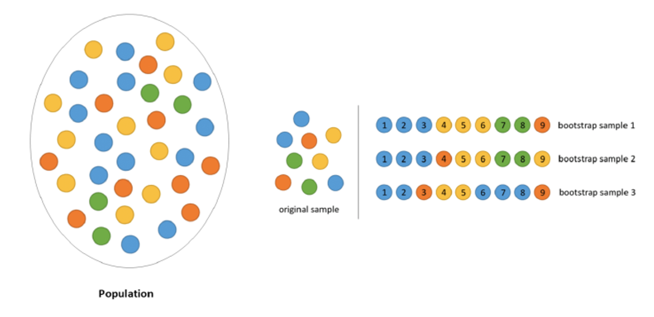
• A bootstrap sample, denoted \(X_1^*,...,X_n^*\), is a sample from a dataset that is drawn with replacement.
• The star notation, \(^*\), is commonly used for to indicate bootstrap samples and estimates from bootstrap samples.

Terminology & notation

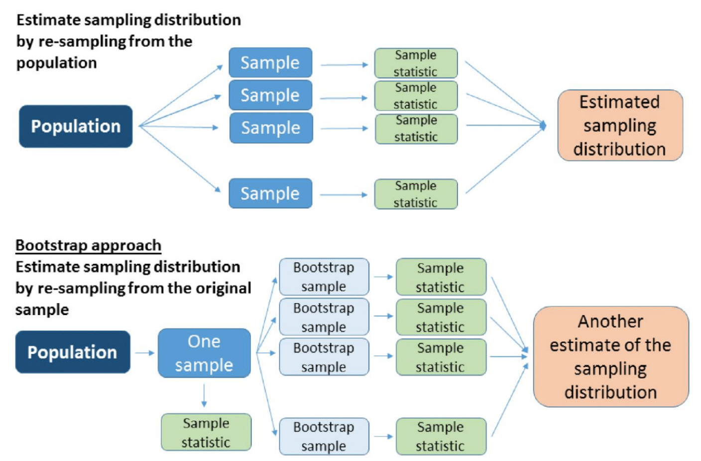
• The estimate \(\widehat\theta_b^*\) is the bootstrap statistic, or bootstrap estimate.
• The distribution of the bootstrap statistic is the bootstrap distribution.

Bootstrap Principle

Approximate the sampling distribution by simulating many datasets from a good model of the distribution of the data and calculate a new estimate of the statistic for each simulated dataset.

• Use the data to compute an estimate of \(\widehat{F}\) of the “true” distribution \(F\).
• Replace the random sample \(X_1,...,X_n\) from \(F\) with a random sample \(X_1^*,...,X_n^*\) from \(\widehat{F}\)
• Approximate the distribution of \(\widehat{\theta}=h(X_1,...,X_n)\) by the distribution of \(\widehat{\theta}_b^*=h(X_1^*,...,X_n^*)\), which is calculated from the random sample.

How to bootstrap

In general

A bootstrap algorithm has the following form:

1. By taking a random sample from the original data, generate a bootstrap sample → \(X_1^*,...,X_n^*\)
2. Calculate the bootstrap statistic from the bootstrap sample → \(\widehat{\theta}^* =h(X_1^*,...,X_n^*)\)
3. Repeat 1. & 2. many times.

Result: Many values of the bootstrap statistic. The distribution of the bootstrap statistic is the bootstrap distribution.

Empirical (or non-parametric) bootstrap

Input

• sample \(X_1,...,X_n\)
• estimator \(\widehat\mu\)
• number of bootstrap samples, \(B\)

Empirical (or non-parametric) bootstrap

Repeat the following for each of \(b=1,...,B\):

1. Sample with replacement from \(X_1,...,X_n\) to obtain a bootstrap sample \(X_1^*,...,X_n^*\)
2. Compute the bootstrap statistic \(\widehat{\mu}_b^*\) from the bootstrap sample

Empirical (or non-parametric) bootstrap

Output

\(\widehat{\mu}_1^*, ..., \widehat{\mu}_B^*\), which are a sample from the sampling distribution of \(\widehat\mu\)

Why “empirical”?

This algorithm is equivalent to sampling from empirical cumulative distribution function. Recall that the eCDF is defined by

\[ \widehat{F}_n(x)=\frac{\big\lvert \{x_i \vert x_i\leq x \} \big\rvert}{n} \]

Why “non-parametric”?

Notice that no parametric family needs to be specified for the distribution.

Example

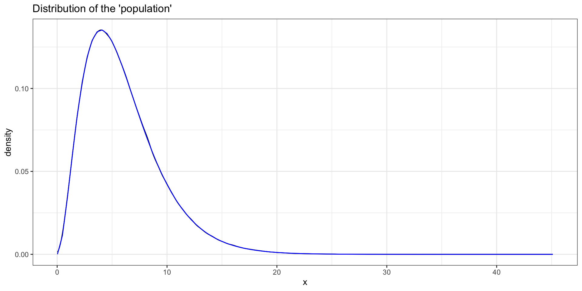
“Population”

set.seed(238)

alpha <- 3
beta <- 0.5

# create a "population"
pop <- rgamma(1000000, shape = alpha, rate = beta)

# compute "true" mean
mu <- mean(pop) 
mu

[1] 6.00168

Is that what we expected?

for \(X \sim \text{Gamma}(\alpha,\beta)\), \(\mathbb{E}[X]=\frac{\alpha}{\beta}\)

Does it look like a Gamma distribution?

ggplot(tibble(x = pop), aes(x = x)) +
  theme_bw() +
  geom_density(color = "black")+
  stat_function(fun = dgamma, args = c( shape = 3, rate = 0.5), color = "blue")+
  labs(title= "Distribution of the 'population'", y = "density") 

Sample

set.seed(238)

n <- 100

# sample from the population
samp <- sample(pop, n, replace = FALSE)

# compute sample mean
muhat <- mean(samp)
muhat

[1] 6.162984

Do we know what the sampling distribution of the sample mean should be for a \(\Gamma\) distribution?

For \(X_1,...,X_n \overset{iid}{\sim} \text{Gamma}(\alpha,\beta)\), \(\bar{X}_n \sim \text{Gamma}(n\alpha, n\beta)\) This can be proven with convolution or MGFs.

Bootstrap (empirical)

set.seed(238)

B <- 1000  # number of bootstrap samples
n <- length(samp)

bootmeans <- numeric(B) # vector where we'll store B bootstrap means

for (i in 1:B){
  bootsamp <- sample(samp, n, replace = TRUE) # sample from the data
  bootmeans[i] <- mean(bootsamp) # compute bootstrap stat
}

# output
ggplot(tibble(x = bootmeans), aes(x = x)) +
  geom_histogram(aes(y = after_stat(density)), bins = 23, colour = "black", fill = "grey") +
  theme_bw() +
  labs(title = "Bootstrap distribution of sample means", y = "density") +
  geom_vline(aes(xintercept = mu), colour = "blue") +
  geom_vline(aes(xintercept = muhat), colour = "purple")

Bootstrap (empirical)

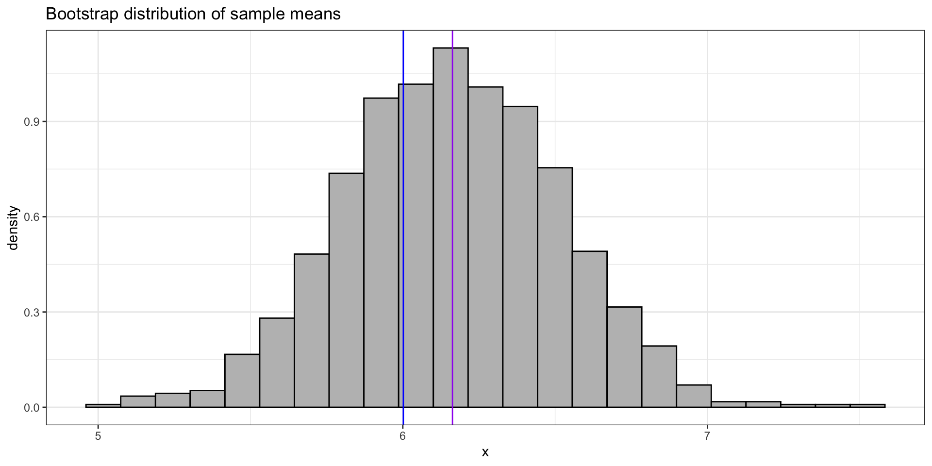
⚠️ The bootstrap does not give a better estimate than the original data because the bootstrap distribution is centered around a statistic calculated from the data. Drawing thousands of bootstrap observations from the original data is not like drawing observations from the underlying population (i.e. the theoretical world). It does not create new data.

How to bootstrap

The bootstrap distribution has approximately the same shape and spread as the sampling distribution, but the center of the bootstrap distribution is the center of the original data (not the center of the theoretical world). So we often use the bootstrap to estimate the sampling distribution of \(\widehat{\theta}-\theta\), the error in our estimate.

Centred estimates

Input

• sample \(X_1,...,X_n\)
• estimate \(\widehat\mu\)
• number of bootstrap samples, \(B\)

Centred estimates

Repeat the following for each of \(b=1,...,B\):

1. Sample with replacement from \(X_1,...,X_n\) to obtain a bootstrap sample \(X_1^*,...,X_n^*\)
2. Compute the bootstrap statistic \(\widehat{\mu}_b^*\) from the bootstrap sample
3. Compute the centered bootstrap statistic \((\widehat{\mu}-\mu)_b^*=\widehat{\mu}_b^*-\widehat{\mu}\)

Centred estimates

Output

\((\widehat{\mu}-\mu)_1^*, ..., (\widehat{\mu}-\mu)_B^*\), which are a sample from the sampling distribution of \((\widehat{\mu}-\mu)\)

We computed \((\widehat{\mu}-\mu)_b^*\) without knowing \(\mu\) (!!)

Example

Bootstrap (centered means)

set.seed(238)

B <- 1000  # number of bootstrap samples
n <- length(samp)

bootcmeans_emp <- 1:B %>%
  map(~sample(samp, n, replace = TRUE)) %>% # sample from the data
  map(~mean(.x) - muhat) %>% # compute bootstrap stat & center
  reduce(c)

ggplot(tibble(x = bootcmeans_emp), aes(x = x)) +
  geom_histogram(aes(y = after_stat(density)), bins = 23, colour = "black", fill = "grey") +
  theme_bw() +
  labs(title = "Centered bootstrap distribution of sample means", y = "density") 

In this course, please do not use the boot package or any other similar packages.

Bootstrap (centered means)

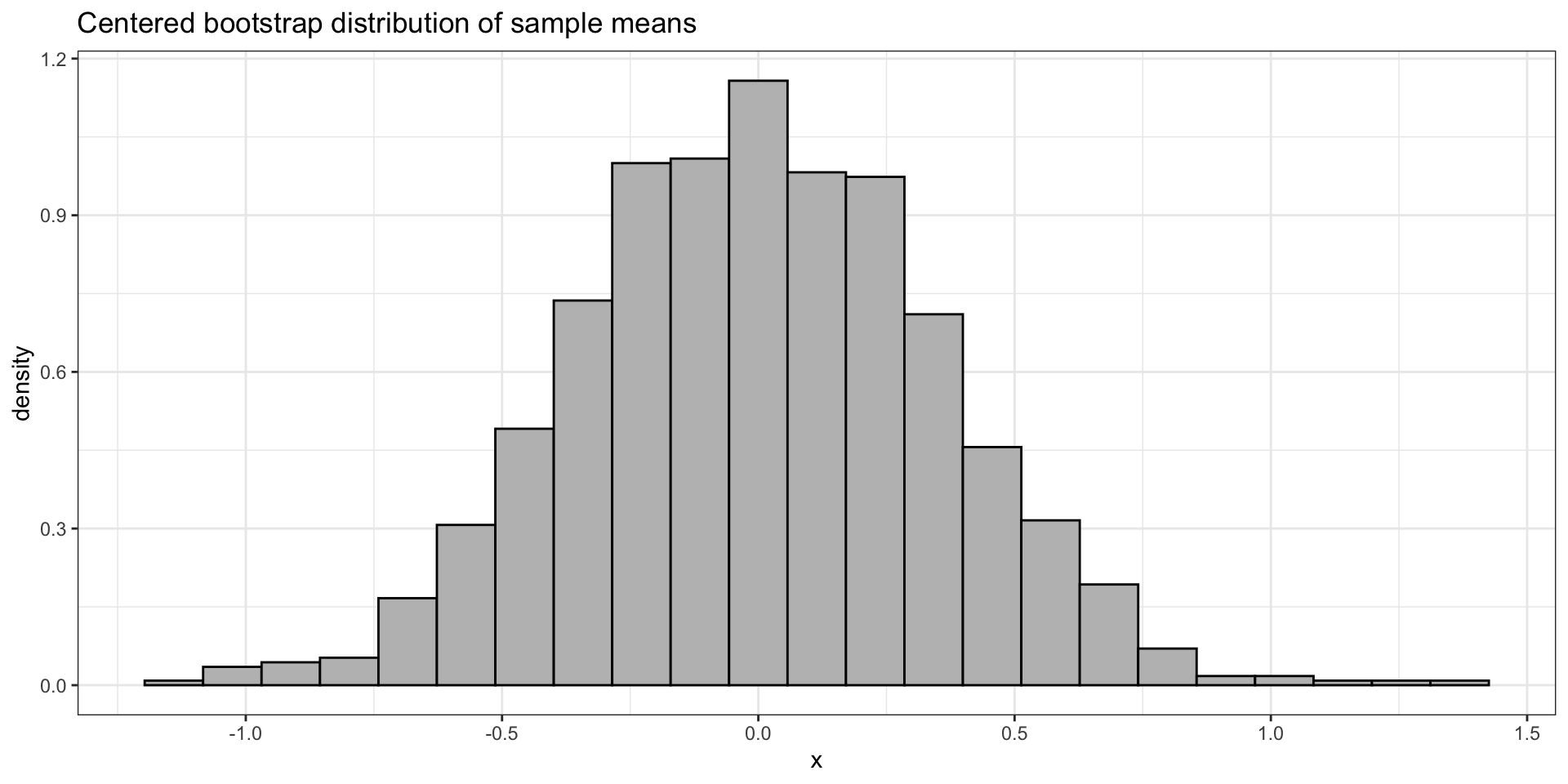
How to bootstrap

Suppose we can make a reasonable assumption about the shape of the distribution of \(F\). Even if it’s not totally correct, it allows the bootstrap to be used in situations where it might fail, particularly for smaller sample sizes.

Parametric bootstrap

Input

• sample \(X_1,...,X_n \overset{iid}{\sim}F_\theta\) where \(F\) is known and \(\theta\) is unknown
• estimate \(\widehat\theta\)
• number of bootstrap samples, \(B\)

Parametric bootstrap

Repeat the following for each of \(b=1,...,B\):

1. Sample from \(F_\widehat{\theta}\) to obtain a bootstrap sample \(X_1^*,...,X_n^*\overset{iid}{\sim}F_\widehat{\theta}\)
2. Compute the bootstrap estimate \(\widehat{\theta}_b^*\) from the bootstrap sample

Parametric bootstrap

Output

\(\widehat{\theta}_1^*, ..., \widehat{\theta}_B^*\), which are a sample from the sampling distribution of \(\widehat\theta\)

Example

Bootstrap (parametric)

set.seed(238)

alphahat <- (mean(samp))^2 / var(samp) # estimate alpha

bootcmeans_par <- numeric(B) # vector where we'll store B bootstrap means

for (i in 1:B){
  bootsamp <- rgamma(n, shape = alphahat, rate = beta) # bootstrap sample with alphahat
  bootcmeans_par[i] <-  mean(bootsamp) - alphahat/beta  # bootstrap estimate
}

What can we do besides plot the sampling distributions?

Bootstrap (parametric)

Estimate \(\widehat\mu-\mu\):

mean(bootcmeans_par)

[1] 0.003870222

… and it’s standard error:

sd(bootcmeans_par)

[1] 0.3249516

What about \(\Pr(|\bar{X}_n-\mu|>1))\)?

mean(abs(bootcmeans_par) > 1)

[1] 0

…and with the empirical bootstrap?

mean(abs(bootcmeans_emp) > 1)

[1] 0.009