Introduction to Bayesian Inference
University of Toronto
July 21, 2023
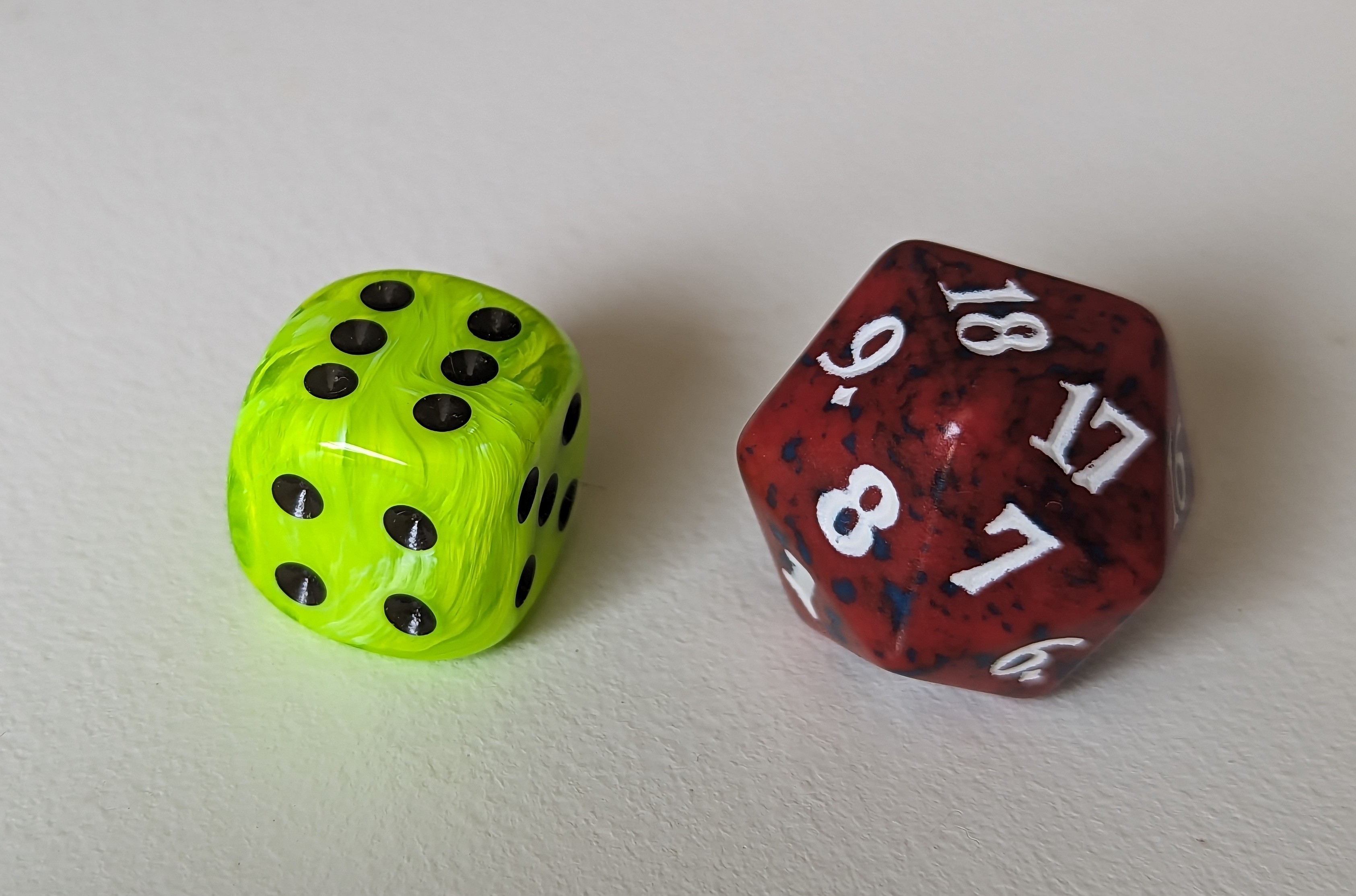
Dice game (revisited)
Recall
🏆 You win if the outcome of the roll of a die is greater than or equal to 5.
6-sided die: \(\frac{1}{3}\)
20-sided die: \(\frac{4}{5}\)
The game
I going to pick one of the dice to roll. You will not know which die I have chosen.
I will roll multiple times, each time reporting whether of not the outcome is a win.
The goal is to come to a consensus about which die I am rolling.
Notation
The outcome is represented by a binary random variable \(W\). \(W=1\) represents a win and \(W=0\) represents a loss.
The parameter \(\theta\) represents which of the dice is rolled. The parameter space \(\Theta\) is \(\{6\text{-sided}, 20\text{-sided}\}\).
A guess
You have no information about how I am choosing a die. What is your best guess for the probability that I will choose the …
…6-sided die?
…20-sided die?
These are called your prior probabilities. They represent what you believe before seeing any data.
An experiment
Let’s collect some data.
| Roll | Outcome |
|---|---|
| 1 | |
| 2 | |
| 3 | |
The analysis
Roll 1
Based on the result of the first roll, what is the probability that I am rolling the 20-sided die?
Want: \[ \Pr(\theta = \text{ 20-sided }|\; W_1= \text{ ___ }) \]
Know:
Our prior probability is \[\Pr(\theta = \text{ 20-sided }) = \text{ ___ }\]
If the 6-sided die was rolled, the probability of the observed outcome is \[\Pr(\; W_1= \text{ ___ } | \theta = \text{ 6-sided })= \text{ ___ }\]
If the 20-sided die was rolled, the probability of the observed outcome is \[\Pr(\; W_1= \text{ ___ } | \theta = \text{ 20-sided })= \text{ ___ }\]
Some theory
Definition 1 (Bayes Rule) \[ \Pr(B_i|A)=\frac{\Pr(A|B_i)\Pr(B_i)}{\Pr(A)} \]
Definition 2 (Law of Total Probability) \[ \Pr(A)=\sum_{i=1}^m \Pr(A|B_i)\Pr(B_i) \] where \(B_1, ...,B_m\) are a partition of the sample space.
Roll 1: Apply theory
By Bayes Rule,
\[ \Pr(\theta = \text{20-sided}| W_1= \text{___ }) = \frac{ \Pr(W_1= \text{ ___ } | \theta = \text{20-sided}) \Pr(\theta = \text{20-sided}) }{ \Pr(W_1= \text{ ___ }) } \]
By the Law of Total Probability,
\[ \Pr(W_1= \text{ ___ }) = \sum_{\theta \in \Theta} \Pr(W_1= \text{ ___ } | \; \theta \; ) \Pr(\theta) \]
Roll 1: Computation
Bayesian terminology
The probability \(\text{P}(\theta = \text{20-sided}| W_1= \text{___ })\) is called a posterior probability.
It combines our initial guess for the probability that the die is 20-sided with the data that we observed, where the data is the result of the first roll.
Combining what we believe a priori (i.e. our prior probabilities) with what we observe from our data is the core of the Bayesian approach to statistics.
We can continue to update our posterior as we observe more data.
Roll 2
\[ \Pr(\theta = \text{20-sided}| W_2= \text{___ }) = \frac{ \Pr(W_2= \text{ ___ } | \theta = \text{20-sided}) \Pr(\theta = \text{20-sided}) }{ \sum_{\theta \in \Theta} \Pr(W_2= \text{ ___ } | \; \theta \; ) \Pr(\theta) } \]
Do we want to update our prior?
Formalizing the Bayesian approach
Parametric statistical model
\[ \{f_{\theta}: \theta \in \Omega \} \]
We want to learn \(\theta\).
Assumes the data was generated by a distribution belonging to a family of distributions, indexed by the parameter.
Bayesian addition
To capture what we might know or believe about the value of the parameter, Bayesian inference uses a probability model for the parameter.
Our “initial guess” for the parameter could be called the prior probability.
Denote the prior probability density function (or, prior probability mass function) as \(\pi(\theta)\).
Applying Bayes Rule
Use Bayes rule to combine the prior probability with the data to get the posterior density function:
\[ \pi(\theta | \mathbf{x})=\frac{f(\mathbf{x}|\theta)\pi(\theta)}{m(\mathbf{x})} \]
where \(m(\mathbf{x})\) is the density function for the marginal distribution of data without dependence on \(\theta\).
Components
Prior : \(\pi(\theta)\)
Data : \(\mathbf{x}=(x_1,...,x_n)\)
Likelihood : \(f_{\theta}(\mathbf{x})\) or \(f(\mathbf{x}|\theta)\)
Marginal : \(m(\mathbf{x})\)
Posterior : \(\pi(\theta|\mathbf{x})\)
Priors
Let \(\theta\) that represents the probability of heads resulting from a coin toss. Note that \(\theta \in \Omega=[0,1]\)
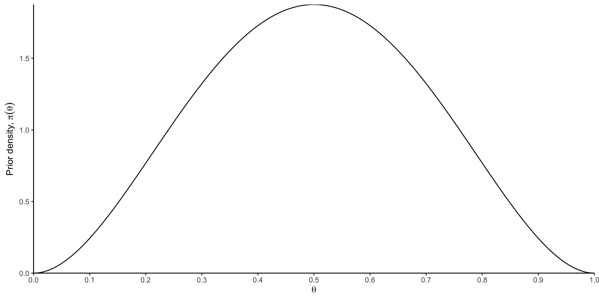


Prior probabilities represent beliefs, not long-run frequencies.
This reflects two fundamentally different interpretations of probability: Bayesian and frequentist interpretations of probability. This is the source of many philosophical debates historically and today.
\[ \; \]
A more practical concern: Where do these beliefs come from in an application? Textbook answer: “from previous experience with the random system under investigation or perhaps with related systems.” While experience is valuable, belief is subjective. Although there may be debates about the philosophical meanings of different approaches to the prior, there are methods for selecting priors that work (beyond the scope of this course).
Likelihood function
Recall from last lecture, \[ L(\theta)= f(x_1|\theta)\times ...\times f(x_n|\theta) \] In the Bayesian context, the notation \(f(\mathbf{x}|\theta)\) is used for the likelihood function. \[ f(\mathbf{x}|\theta)= f(x_1|\theta)\times ...\times f(x_n|\theta) \]
Since \(\mathbf{x}\) is observed, \(f(\mathbf{x}|\theta)\) is a function of \(\theta\).
Marginal density function
To calculate \(m(\mathbf{x})\), integrate (or sum) over any other variable(s) in the joint distribution.
Continuous \[ m(\mathbf{x})=\int_{\Omega} \pi(\theta)f(\mathbf{x}|\theta) d\theta \]
Discrete \[ m(\mathbf{x})=\sum_{\theta \in \Omega} \pi(\theta)f(\mathbf{x}|\theta) \]
Which rule is used in these definitions?
The role of \(m(\mathbf{x})\) is to ensure that \(\pi(\theta|\mathbf{x})\) integrates (or sums) to 1, making the posterior a valid density function — \(m(\mathbf{x})\) is a normalizing constant.
Dice game, formally
Model
\[ W_i \sim \text{Bernoulli}(\theta) \]
The parameter is \(\theta\). The parameter space \(\Theta = \left\{\frac{1}{3}, \frac{4}{5}\right\}\).
Prior
\[ \pi(\theta) = \Pr(\theta = q) = \alpha*{\mathbb{1}_{\theta}(q=1/3)}+(1-\alpha)*{\mathbb{1}_{\theta}(q=4/5)} \]
What value of \(\alpha\) did we use?
Likelihood
\[ p(\mathbf{w}|\theta) = \prod_{i=1}^n p(w_i|\theta) = \theta^{\sum w_i} (1-\theta)^{n-\sum w_i} \]
For the data we observed, the likelihood is
\(m(\mathbf{x})\) does not always need to be computed
[Example 7.1.1 from E&R] Suppose that we observe a sample \((x_1,...,x_n)\) as realizations of a random sample \(X_1,...,X_n\) such that \(X_i\sim Bernoulli(\theta)\). We don’t know \(\theta\), but \(\Theta = [0,1]\) so a Beta distribution is a good prior. What is the posterior distribution?
pdf of a Beta distribution:
\[ f(y)=\frac{\Gamma(\alpha+\beta)}{\Gamma(\alpha)\Gamma(\beta)}y^{\alpha-1}(1-y)^{\beta-1} \;\; \text{for} \;\; 0 \leq y \leq 1 \] where \(\Gamma(\cdot)\) is the Gamma function (a special integral).
Bayes Rule, simplified
The posterior of \(\theta\) is proportional to the likelihood times the prior.
\[ \pi(\theta | x) \propto f(x|\theta)\pi(\theta) \]
When the posterior distribution is from the same distribution family as the prior, we say the prior is conjugate with the likelihood.
Example: Conjugate priors
Consider a gamma distribution with the shape-rate parametrization.
pdf:
\[ f(x)= \frac{\beta^\alpha}{\Gamma(\alpha)}x^{\alpha-1}e^{-\beta x}, \quad x>0, \quad \alpha,\beta>0 \] where \(\Gamma(\cdot)\) is the Gamma function, \(\alpha\) is shape parameter, and \(\beta\) is a rate parameter. Suppose that random variables \(X_1,\dots X_n\) are conditionally independent given \(\beta\), that is, \[ X_i | \alpha,\beta \sim \text{Gamma}(\alpha,\beta) \]
Suppose that \(\alpha>0\) is known, and that the \(\beta\) has the prior distribution \[ \beta \sim \text{Gamma}(\alpha_0,\beta_0) \] Show that this prior is conjugate with the likelihood.