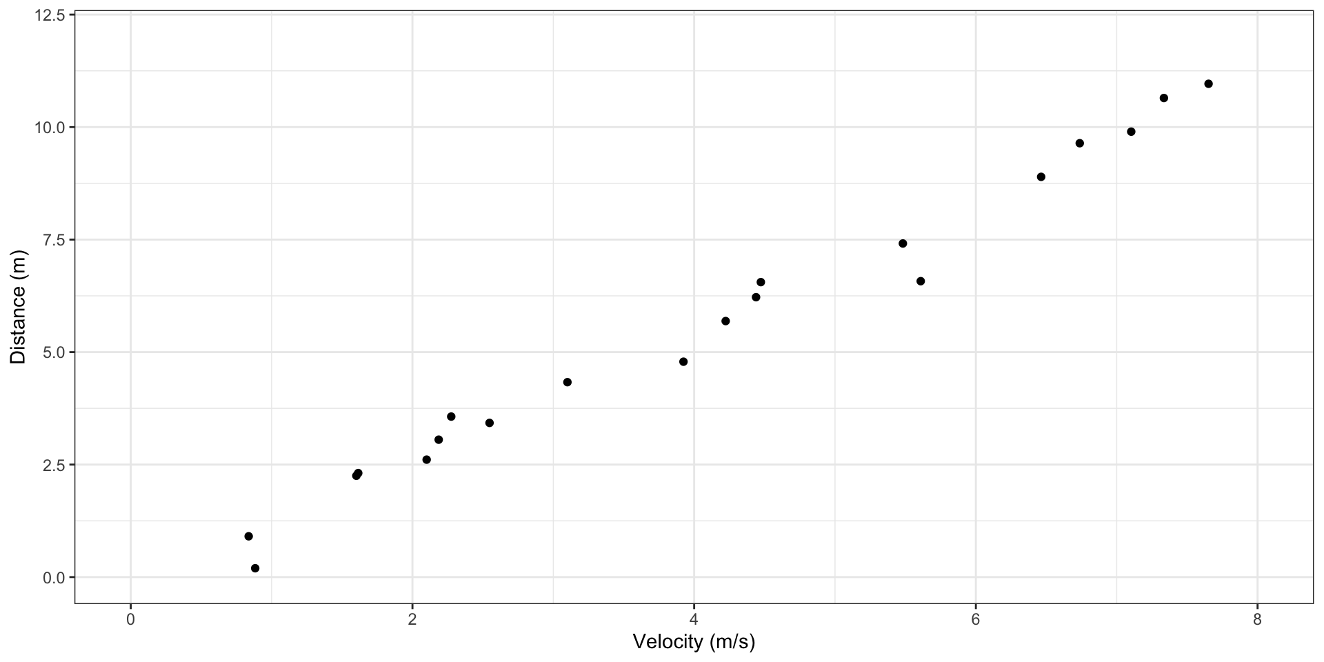
plot_flights <- ggplot(data = paperflights, aes(x = v, y = d)) +
  theme_bw() +
  coord_cartesian(xlim = c(0,8),ylim = c(0,12)) +
  geom_point() +
  labs(x = "Velocity (m/s)", y = "Distance (m)")
plot_flights
University of Toronto
July 12, 2023
The sciences do not try to explain, they hardly even try to interpret, they mainly make models. By a model is meant a mathematical construct which, with the addition of certain verbal interpretations, describes observed phenomena. The justification of such a mathematical construct is solely and precisely that it is expected to work - that is correctly to describe phenomena from a reasonably wide area. Furthermore, it must satisfy certain esthetic criteria - that is, in relation to how much it describes, it must be rather simple.
~ John von Neumann


This is a deterministic model. Nothing is random.
A statistical model is an idealization of the data-generating process, or an abstraction describing how out data came about.
Statistical models always involve stochasticity, that is, an element of randomness.
All models are wrong, but some are useful.
~ George Box
We make repeated measurements of the same quantity and collect the observations in a dataset, denoted \(x_1, x_2, ...,x_n\). The observations are modelled as the realization of the random sample \(X_1, X_2, ...,X_n\).
A random sample is a collection of random variables \(X_1, X_2, ...,X_n\) that have the same probability distribution and are mutually independent. That is, \[X_1, X_2,..., X_n \overset{iid}{\sim} F\]
The statistical model is \(F\), the probability distribution of each \(X_i\).
The unique distribution that the sample is drawn from is called the “true” distribution.
Parameters are an unknown element of a statistical model for observable data. They represent unobservable or unknown properties that we want to know about.
A parametric model has a partial specification of the probability distribution of \(F\). \[ \{F_{\theta }:\theta \in \Theta \} \]
The parameter value(s) that specify the true distribution are called the “true” parameter(s).
Consider a statistical model \(X_i \sim {N}(\mu,\sigma^2)\).
Recall: LLN
The sample mean \(\bar{X}_n\) converges in probability to \(\mathbb{E}[X_i]=\mu\), the true mean, provided that \(\text{Var}(X_i) = \sigma^2 < \infty\). This is written as \[ \bar{X}_n \overset{p}{\longrightarrow} \mu \]
The LLN shows that the sample mean gets close to the expectation of a probability distribution.
The sample mean, \(\bar{X}_n\) is an example of a sample statistic.
A sample statistic is an object which depends only on the random sample \(X_1, X_2, ...,X_n\): \[ h(X_1, X_2, ...,X_n) \]
A realization of this sample statistic would be \(h(x_1, x_2, ...,x_n)\).
For large sample size n, the sample mean of most realizations of the random sample is close to the expectation of the corresponding distribution.
Exercise 1 Let \(X_i \overset{iid}{\sim} F_{\mu ,\sigma^2} , \;i = 1, ..., n\) be a random sample from an unknown distribution \(F_{\mu ,\sigma^2}\) with parameters \(\mu = \mathbb{E}[X_i]\) and \(\sigma^2 = \text{Var}(X_i)\). Suppose we estimate the population variance \(\sigma^2\) using the “known mean” sample variance:
\[ \widetilde{s}_n^2 = \frac{1}{n} \sum_{i=1}^{n}( X_i − \mu )^2 \]
Show that \(\widetilde{s}^2_n \overset{p}{\rightarrow} \sigma^2\). What conditions are required on \(X_i\) for this to be true?
Say we wanted to predict the horizontal distance a paper airplane flies based on initial horizontal velocity. We could write this as:
\[ \text{distance}=g(\text{velocity}) \]
But there are other possible factors. Add a random component to account for the unknown:
\[ \text{distance}=g(\text{velocity})+\text{random fluctuation} \]
How do we know which plot would be useful here?
The data look reasonably linear. So we can represent the model as:
\[ \text{distance}= \alpha + \beta * (\text{velocity}) + \text{random fluctuation} \]
This is a simple linear regression model.
Consider bivariate data \((x_1,y_1), ...,(x_n,y_n)\). In simple linear regression, we assume \(x_1,...,x_n\) are fixed (not random) and that \(y_1,...,y_n\) are realization of random variables \(Y_1,...,Y_n\) such that
\[ Y_i= \alpha + \beta x_i + U_i \;\; \text{for} \;\; i=1,...,n \]
where \(U_1, ...,U_n\) are independent random variables with \(\mathbb{E}[U_i]=0\) and \(\text{Var}(U_i)=\sigma^2\).
\(y=\alpha + \beta x\) is called the regression line.
\(\alpha\) and \(\beta\) represent the intercept and slope, respectively.
\(\alpha\) and \(\beta\) are the model parameters.
\(y\) is the response variable or the dependent variable
\(x\) is the explanatory variable or the independent variable
Simple linear regression means the model has 1 explanatory variable. If there are multiple explanatory variables, then it is multiple linear regression.
Call:
lm(formula = d ~ v, data = paperflights)

Coefficients:
(Intercept)            v
-0.3167 1.4428 Independent & \(\mathbb{E}[U_i]=0\)
⇒ \(Y_i\)’s are equally far away from the line and are scattered about the line in a random way
\(\text{Var}(U_i)=\sigma^2\)
⇒ same amount of scatter or variability about the line everywhere
What would the scatterplot look like if the conditions on \(\{U_i\}\) were violated?
\(Y_1,...,Y_n\) are independent, but not identically distributed.
\(U_1, ...,U_n\) are independent \(\implies\) \(Y_1,...,Y_n\) are independent
To verify, consider \(\mathbb{E}[Y_i Y_j]\).
How do we know that \(Y_1,...,Y_n\) are not identically distributed?
\[ \mathbb{E}[Y_i]=\alpha + \beta x_i + \mathbb{E}[U_i]=\alpha + \beta x_i \] They have different means!