Exploratory Data Analysis

Sonia Markes

University of Toronto

July 6, 2023

• A probability is a number between 0 and 1 indicating how likely an event is, whereas a statistic is a number in a context.
• Say you have a list of numbers, denoted \(x_1, x_2, ..., x_n\). These are (observed) data values.
• We conceptualize them as realizations of random variables \(X_1, X_2, ...,X_n\).

The data do not speak for themselves.

Numerical Summaries

• Center
• Order statistics
• Variability

Center

• Sample Mean
• Sample Median

Sample Mean

\[ \bar{x}_n = \frac{x_1+x_2+...+x_n}{n} \]

The arithmetic mean, or simply, the average. Denoted \(\bar{x}_n\) or, simply \(\bar{x}\).

Sample Median

The sample median is the middle value of a sorted dataset. Denoted \(Med_n=Med(x_1,x_2,...,x_n)\).

• If n is odd, the median is an element of the dataset.
• If n is even, the median is the average of the middle two values.
• Roughly, half the data is above the median, and half is below.

Exercises

Find the mean and median of the following sets:

1. \(\{ 6,4,7,5,3\}\)
2. \(\{3,5,9,2,4,7\}\)
3. \(\{7,8,8,1\}\)

Ex 1: Find the mean and median of \(\{ 6,4,7,5,3\}\)

ex1 <- c(6,4,7,5,3)
n1 <- length(ex1) 
sum(ex1) / n1 # mean
sort(ex1)[ (n1+1)/2 ] # median 

Ex. 2: Find the mean and median of \(\{3,5,9,2,4,7\}\)

ex2 <- c(3,5,9,2,4,7)
n2 <- length(ex2)
sum(ex2) / n2 # mean
quantile(ex2, prob=0.5) # also median 

Ex. 3: Find the mean and median of \(\{7,8,8,1\}\)

ex3 <- c(7,8,8,1)
mean(ex3)
median(ex3)

Comparison

• Mean of a dataset \(\sim\) Expectation of a probability distribution, \(\mathbb{E}[X]\)
• Median is less sensitive to outliers, that is, to the few values that are far from most of the values.

Order

• Notation
• Empirical Quantiles

Order statistics

The dataset arranged is ascending order is called the order statistics, denoted \(\{x_{(1)},x_{(2)},...,x_{(n)}\}\), such that \[x_{(k-1)}\leq x_{(k)}\leq x_{(k+1)} \;\; \forall \;\; k\in(1,n)\]

Special cases

\[ \min (x_1, ..., x_n) =x_{(1)} \]

\[ \max (x_1, ..., x_n)=x_{(n)} \]

Median, revisited

\[ {Med}_n = \begin{cases} x_{\left(\frac{n+1}{2}\right)} &\text{if } n \in 2k+1 \\ \frac{1}{2} \left( x_{\left(\frac{n}{2}\right)} + x_{\left(\frac{n}{2}+1\right)} \right) &\text{if } n \in 2k \end{cases} \] where \(k\in \mathbb{N}\)

Empirical Quantiles

The \(p^{th}\) empirical quantile, denoted \(q_n(p)\), is the number such that the proportion of the dataset below \(q_n(p)\) is \(p\).

Special cases

• The median is the \(0.5^{th}\) empirical quantile, or \(q_n(0.5)\).
• Percentile:
  • \(x^{th}\) percentile = \(p^{th}\) quantile, where \(x=p \times 100\)
• Quartiles:
  • Lower quartile = \(q_n(0.25)\)
  • Upper quartile = \(q_n(0.75)\)

Five-number summary

1. Minimum
2. Lower quartile
3. Median
4. Upper quartile
5. Maximum

Exercises

For the set of integers \([1,11]\), compute the following:

1. \(10^{th}\) percentile
2. Five-number summary

ex_order <- 1:11
quantile(ex_order, p = 0.1) # 10th percentile
c(min(ex_order), 
  quantile(ex_order, 0.25),
  median(ex_order),
  quantile(ex_order, 0.75),
  max(ex_order)) # 5-number summary

Variability

• Range
• Deviation

Ranges

The range of a dataset is the difference between the maximum and minimum values. \[ Max-Min=x_{(n)}-x_{(1)} \]

The interquartile range is the difference between the upper and lower quartiles. \[ IQR = q_n(0.75) - q_n(0.25) \]

About a center

Median of absolute deviation

\[ MAD(x_1,...,x _n)= Med\left( |x_1-Med_n|,...,|x_n-Med_n| \right) \]

Sample variance

\[ s_n^2 = \frac{1}{n-1}\sum_{i=1}^n (x_i-\bar{x}_n)^2 \] The sample standard deviation is \(s_n\), the square root of the sample variance.

Why \(n-1\)? Intuition: If I know \(\bar{x}\), then I only need \(n-1\) data points in order to know the value of the \(n^{th}\) data point.

Exercises

Compute the range, interquartile range, MAD, and standard deviation for \(100\) observations from the following distributions:

1. \(W \sim U(0,1)\)
2. \(X \sim N(0,1)\)
3. \(Y \sim Exp(1)\)

# Set the number of observations
n <- 100

\(W \sim U(0,1)\)

set.seed(111)
w <- runif(n, min = 0, max = 1) 

max(w) - min(w) # range

[1] 0.9957914

quantile(w, 0.75) - quantile(w, 0.25) # IQR

      75% 
0.3884707 

median( abs(w - median(w)) ) # MAD

[1] 0.184963

sd(w) # standard deviation

[1] 0.2757188

\(X \sim N(0,1)\)

set.seed(111)
x <- rnorm(n, mean = 0, sd = 1)

max(x) - min(x) # range

[1] 5.831273

quantile(x, 0.75) - quantile(x, 0.25) # IQR

     75% 
1.353497 

median( abs(x - median(x)) ) # MAD

[1] 0.7001285

sd(x) # standard deviation

[1] 1.070855

\(Y \sim Exp(1)\)

set.seed(111)
y <- rexp(n, rate = 1)

max(y) - min(y) # range

[1] 7.029369

quantile(y, 0.75) - quantile(y, 0.25) # IQR

      75% 
0.9481848 

median( abs(y - median(y)) ) # MAD

[1] 0.4223345

sd(y) # standard deviation

[1] 1.197168

Graphical Summaries

• Boxplots
• Histograms
• Kernel density estimates
• Empirical cumulative distribution function
• Scatterplots

Box-and-whisker plot

Features of boxplots

• Based on 5-number summary.
• Box covers the interquartile range, with the median indicated.
• Dots indicate outlier data points.
• “Whiskers” extend to the extremal data points that are not outliers.

Outliers

One method of defining outliers is to use the IQR measure of variability.

\[ x_i\leq q_n(0.25) - 1.5*IQR \]

\[ x_i \geq q_n(0.75) + 1.5*IQR \]

What do boxplots show?

• Location of the median
• Dispersion
• Outliers
• Symmetry or skewness

What do boxplots not show?

• Gaps in the data
• Multiple modes

Histogram

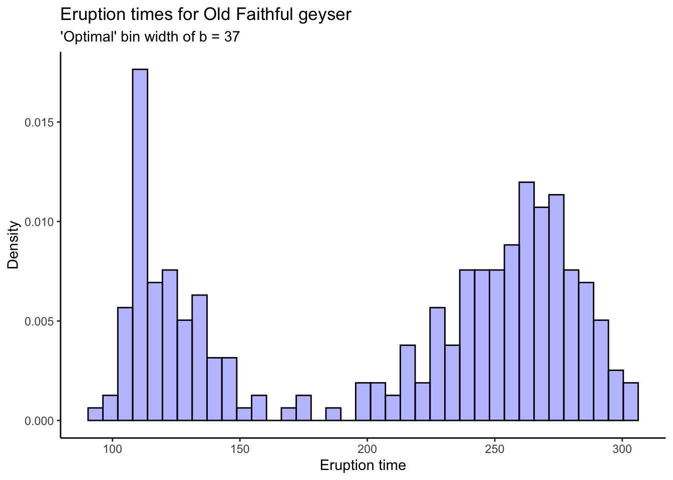
Bins

Put data into \(m\) bins, \(B_1, ..., B_m\), \[ B_i=\left[x_0+(i-1)b, \;x_0+ib\right) \] where \(b\) is the bin width.

• The area under the histogram on a bin \(B_i\) is the proportion of data points in \(B_i\).
• The height of the \(i^{th}\) bin is the proportion of data points in \(B_i\) divided by the bin width \(b\).
• Note: \(x_0\) does not need to be in the dataset.

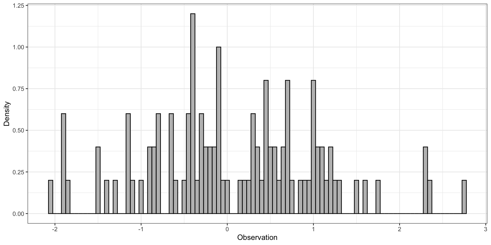
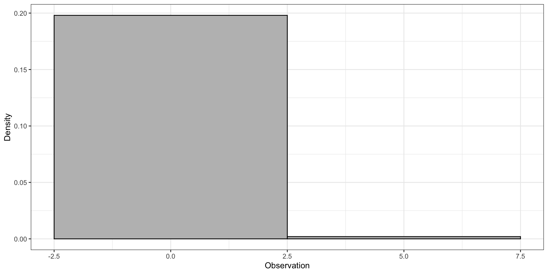
Bin width can impact what we can learn from a histogram.

Example

library(tidyverse)
set.seed(2023)
df <- tibble(
  x = rnorm(n = 100, mean = 0, sd = 1) # generates data
  ) 

Too small ⇒ too noisy

df %>%
  ggplot(aes(x = x)) + 
  theme_bw() +
  geom_histogram(aes(y=after_stat(density)), 
                 colour = "black", fill = "grey", 
                 binwidth = 0.05) +
  labs(x = "Observation", y = "Density")

Too big ⇒ lose features of the data

df %>%
  ggplot(aes(x = x)) + 
  theme_bw() +
  geom_histogram(aes(y=after_stat(density)), 
                 colour = "black", fill = "grey", 
                 binwidth = 5) +
  labs(x = "Observation", y = "Density")

“Optimal” bin width

b <- (24*sqrt(pi))^(1/3) * sd(df$x) * (length(df$x)^(-1/3)) # Rmk 15.1 [MIPS]
df %>%
  ggplot(aes(x = x)) + 
  theme_bw() +
  geom_histogram(aes(y=after_stat(density)), 
                 colour = "black", fill = "grey", 
                 binwidth = b) +
  labs(x = "Observation", y = "Density")

Shapes

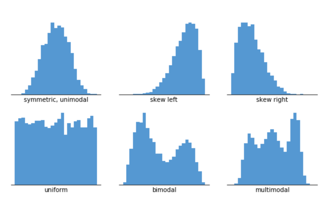
What do histograms show?

• Location of centre or typical value(s)
• Number of typical value(s) or “peaks”
• Variability about typical value(s)
• Symmetry (or skewness)
• Gaps or outliers in data

With appropriate scaling of the height of the bins, histograms can be a crude estimate of an unknown probability density \(f\) under which the data was generated.

Density estimate

Histogram vs KDE

• Similar to (scaled relative frequency) histogram, a kernel density estimate, \(f_{n,h}(t)\), is an estimate of an unknown probability density \(f\) under which the data was generated.

• Unlike a histogram, a KDE is smooth. Instead of weighting each datapoint by \(1/n\), a density function called a kernel is used to weight each datapoint.

• Intuition: A histogram is like stacking bricks. A KDE is like piling up sand. (Helpful demo 🔗)

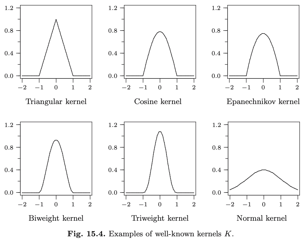
Kernel, \(K(t)\)

Reflects the shape of the sand pile. Choose a shape.

Properties of kernels

1. \(K(t)\) is a probability density, that is, \(K(t)\geq 0\) and \(\int_{-\infty}^{\infty} K(t) dt =1\).

2. \(K(t)\) is symmetric about zero, that is, \(K(t)=K(-t)\).

3. [often] \(K(t)=0\) for \(|t|>1\).

Bandwidth, \(h\)

• Reflects the width of the pile of sand.

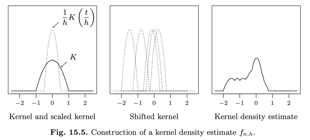
• Scale the kernel by \(h\). \[ t \mapsto \frac{1}{h}K\left( \frac{t}{h}\right) \]

• Bandwidth controls the smoothness.

Constructing a KDE

To compute \(f_{n,h}(t)\), shift the scaled kernel to each data point and take the average

\[ f_{n,h}(t)=\frac{1}{n}\left\{ \frac{1}{h} K\left( \frac{t-x_1}{h}\right) + ... + \frac{1}{h} K\left( \frac{t-x_n}{h}\right) \right\} \]

What do KDEs show?

• Location of centre or typical value(s)
• Number of typical value(s) or “peaks”
• Variability about typical value(s)
• Symmetry (or skewness)
• Gaps or outliers in data

Empirical distribution

eCDF

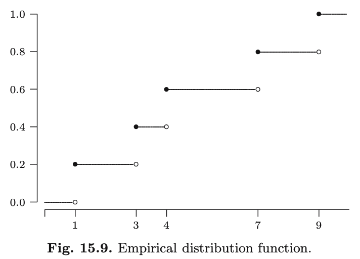
The empirical (cumulative) distribution function, or, eCDF, is defined by \[ F_n(x)=\frac{\big\lvert \{x_i \vert x_i\leq x \} \big\rvert}{n} \]

Example

Consider the dataset: \(\{4,3,9,1,7\}\)

What do eCDFs show?

• An estimate of the unknown cumulative distribution function under which the data was generated.

What is the relationship between the eCDF and kernel density estimator?

Exercise: MIPS ~15.11

Suppose you have a histogram and an empirical distribution function \(F_n\) for the same dataset. Derive an expression for the height of the histogram on the bin \((a,b]\) in terms of \(F_n\), \(a\), and \(b\).

1. area under the histogram on the bin \((a,b]\)
2. height of the histogram
3. \((a,b] = (0,b]-(0,a]\)
4. recall definition of ecdf

Scatterplot

Bivariate data

• So far, we’ve only considered univariate data, that is, data with only one variable.

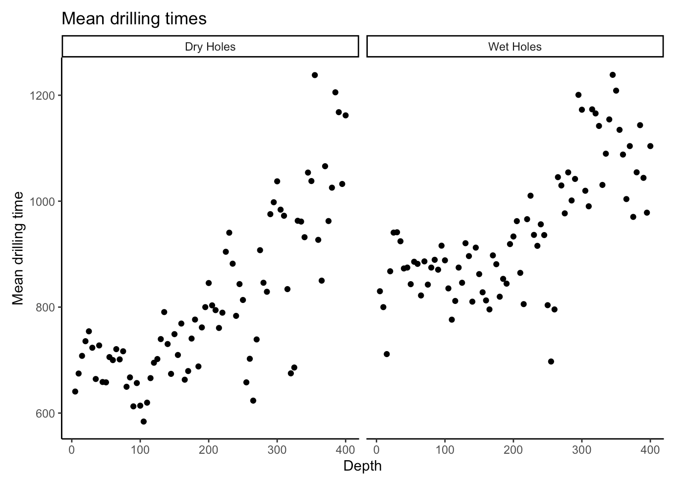
• If we have pairs of datapoints, \(\left\{(x_1,y_1),...,(x_n,y_n)\right\}\), the data is called bivariate.

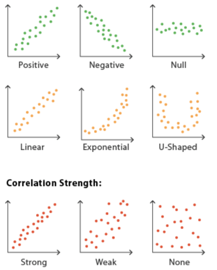
• Scatterplots are used to investigate the relationship between variables.

What do scatterplots show?

• Direction
• Shape
• Correlation strength (sometimes)

Choosing a visualization

• Histograms are usually a good idea, at least as a first look.
• Kernel density estimates and eCDFs are usually a good idea if you have the computing resources, especially if want to learn about the distribution or the data-generating process.
• Boxplots are good for comparing multiple variables/datasets that are each unimodal.
• Scatterplots are good for investigating the relationship between two or more variables.
• Or, try all appropriate visualizations and then choose!